Lossy compression can be driven by two factors: acceptable reciprocal noise level q, 0 <= q <= 1, and compression strength ratio, rc, 0 <= rc <= 1. We will apply image blur as a function of q and image decomposition as an inverse function of rc. (I.e., image decomposition will produce a minimized value of rc, for an image blur controlled by q.)
1. Image blur
If one is driving a car at high speed and observing at a constant angle w, with w = 0 corresponding to the vanishing point of the road at the horizon, w = pi/2 corresponding to the left right angle to the road, and w = -pi/2 corresponding to the right right angle to the road, then one will have a clear picture of image blur. At a certain value of w, there is a limit to the maximum amount of information available at the viewing rate of one's eyes.
If one could take a snapshot of the information viewed on the roadside at w = pi/2, there would be just as many picture elements (pixels) as the snapshot recorded at w = 0. The picture of the road straight ahead is very clear, but the vehicle's motion obscures one's view of the roadside, when observed from a constant angle and not tracked by eye movement. If image motion exceeds the size of one pixel, then increasing the resolution (or in analogy, increasing the quality by reducing compression strength) does not provide more image information.
This analogy to image blur is used to clarify the following description of iterative refinement. Suppose that we continually increase the precision (or discrete "resolution") of the image; for w = 0, this will continuously provide more image information. For w != 0, this process of providing more resolution will provide more resolution, of course, but it will not keep continuing to provide more image information. Image motion prohibits the average image information from increasing beyond a certain limiting value, no matter what the resolution.
To illustrate this concept we plot a function converging to 0 (representing the image error as resolution increases or as relative compression reduction decreases, and a function converging to 0 plus different levels of random noise).
% ./pngplot '[0:100] y(x,z) = sin(x)/(x*(x+1)**.2)+z*rand(0)-z/2, y(x,0), y(x,.05),y(x,.1),y(x,.5)' sinx-x.png
![[0:100] y(x,z) = sin(x)/(x*(x+1)**.2)+z*rand(0)-z/2, y(x,0), y(x,.05),y(x,.1),y(x,.5)](sinx-x.png)
The function y(x, z) uses z as a motion parameter, where z is approximately tan(w). One can see that it is useless to try to reduce the error tolerance below the value of z. Thus, it is best to compress as much as possible while any compression errors are still hidden below the value of blur in the picture.
But to do this, one needs an algorithm.
Algorithm 1.1. Reduction of blur.
function y = blur1(x, f)
p0 = 0;
     y = f(x, p0);
  err = relerr(x,y); % from 0 to 1.
err0 = 1;
tic

while toc < 0.5
p0 = p0 + (1-p0)*err;
err0 = err;
y2 = f(x, p0);
err = relerr(x,y2);

if err >= err0*p0
break;
else
y = y2;
end

end
This function actually defines a new compression algorithm which will start at quality 0. The quality will be increased until it falls within the quality level of the original random noise. This will automatically find a rough approximation to the point where the image blur exceeds the compression blur. (This is done by based on the expected value of how much relative quality increase should be caused by a certain increase in the inverse parameter rc. Based on the first approximation to the image, allowing rc to increase should allow the value of q to decrease by a certain amount. When this does not occur, the blur of the image is judged to exceed the value of compression error, as is represented by the jiggles in the graph of y(x, z), where the noise will always cause the effective value of q to be >= z, and so there is no point in reducing the computed q to be any less than c.)
(Also note that it is easy to write compression algorithms for which compressing to quality level 0 requires less computation, and so these initial approximations require very little work. In particular, constant images will be completed in precisely one step. Thus, this method meets one of the design criteria for a "reasonable algorithm," that easy things should not be harder to do than hard things.)
To illustrate this, imagine a picture consisting of random pixels. Increasing the compression quality somewhat will not result in as large of a change in "quality" relative to the original image, because the image is so random. In fact, since the image is so random, it almost makes no difference how much compressed the image is. So the blur algorithm will allow the image to be compressed very greatly, since it doesn't matter, whereas most compression algorithms would be unable to compress the image at all since it consists of random information.
2. Decomposition
To hide compression errors below the value of blur, it also helps if one could decompose the image into portions where there is a great deal of blur, compression errors are hidden, and compression can be high (rc very low). For example, it is nice to see people clearly in a picture, but the elements in the blue sky can be incorrectly positioned, and it remains the same color of blue and maintains the same appearance.
So we can imagine it would be helpful to isolate the similar parts of an image and then apply a compression algorithm to the level of blur present in only that portion of the image. Thus, most of many images could be compressed highly, while important shapes were carefully detailed and high quality. (This is the idea of "variable quantization.")
The discussion of decomposition is continued in
Lossy Image Compression and Decomposition for Continuous-tone Images
3. Measuring the value of rc
We can assume that a compression function is defined like this:
function [y,cost] = linearc1(x, r)
% tries to pretend like the function
% is evenly changing across the whole plane;
% the decomposition will break the image
% into partitions making the compression
% work by assuming that the image is
% a solution to the Laplace equation,
% and each pixel is the average of its
% neighbors.
[m,n] = size(x);
v0 = x(1,:);
cost = n;
cover = n;

y(i,:) = v0;

for i=2:m
cover = cover + n;
if cost/cover > r
cost = cost + 1;
coef = mean(x(i,:))/mean(v0);
y(i,:) = v0*coef;
else
cost = cost + n;
v0 = x(i,:);
y(i,:) = v0;
end
This completely allows us to determine the value for compressing an image A with this compression function:
[B,cost] = linearc1(A, rcapprox);
rcexact = cost/originalsize;
For counting the value of rc for a decomposed image, we can assume that each decomposed image requires one pixel value plus its own size.
In storage, the decomposed image can be represented by any initial cell, plus an extra pixel which "stores" the coordinates of the next cell, and so on inductively. This is nothing more than a linked-list, and obviously, the decompressed image should be saved internally for graphics processing while it is needed. Then the unnecessary cost of re-traversing the linked list of cells is avoided. But this is only the same as saying that we want to save the cost of computing something twice, which applies to any kind of decompression.
We'll take an example image:

Now compressing it by linearc as a function of rc, we can define:
function [y,cost] = imagefuncapply(x, func)
% applies a function to each of the three
% color planes
[n, m, p] = size(x);
y = double(x)/255;
c = zeros(p);
for i=1:p
    [y(:,:,i),c(i)] = feval(func, y(:,:,i));
end
y = max(0, y);
y = min(1, y);
y = uint8(y*255);
cost = sum(c);
and then we perform:
x = imread('iris.jpg');
[y,cost] = imagefuncapply2(x, @linearc1);
rc = cost/prod(size(y);
After starting life as a JPEG image and being decomposed into a number of rectangles, based on a total of 28686/944784 singular points, the resulting compression strength was rc = 0.523. The actual representation is 1/4th of the original image storage space (yk = 4), but due to the cost of the image storage structure, the total savings is slightly less than 1/2.
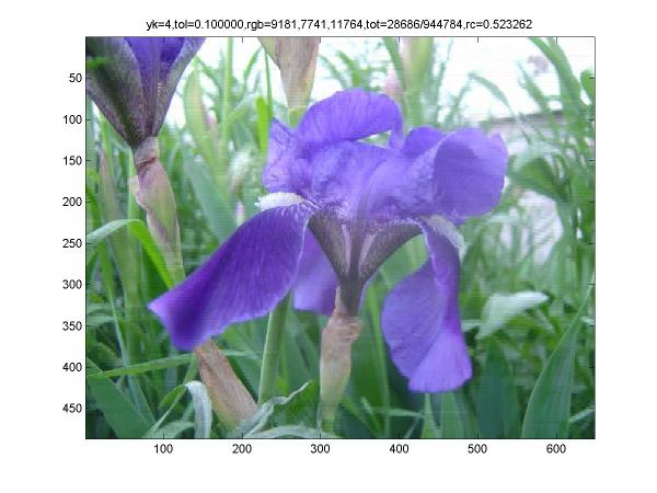
When blur is factored in, the compression increases, and the actual representation is 1/3rd of the original image, and the number of singular points reduces to 15,253, with rc = 0.479.

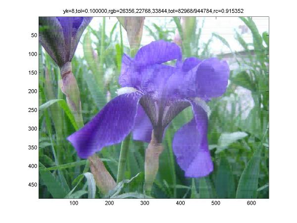
An overcompressed example reduces the image from its original size by more than 1,000 percent, but the result is only useful in analying the visual effects of this algorithm.

Now we will observe the result of increasing accuracy below the origial blur level of the image: compressed size starts to increase (rc = 0.915) after reaching its minimum value (corresponding to rc = 0.479).
References:
1. Myers JK. Programming Style and Wasted Indentation. 2001. CJM.
2. Myers JK. Reentrant Algorithms and the General Usefulness of Time. 2005.
3. Myers JK. The Use of toc in While Loops. 2005. (for Matlab).
Excerpts:
[2]
[Reentrant Algorithms]: "... such an algorithm can be stopped, started, or continued as easily as walking, stopping, and continuing to walk, and with just as little concern for the details." (Example: readhdr() in libheaders.)