Continuous-tone images
In this discussion, we may assume that images are represented in a subset of 48-bit color, and that matrices of the image consist of evenly scaled luminosity values, with the whole image formed by the superposition of red, green, and blue separated additive color planes.
A continuous-tone image is characterized by containing connected areas of gradually changing luminosity, except at a relatively small number of exceptional points, which are collectively referred to as edges or corners.
Several similar words are used to refer to this points. In particular, a singular point has the sense of a point in the image which is not continuous. Thus, for a continuous image, such a point is a singularity.
Determining corners and edges
Our definition of discontinuous points--and its implied definition of corners and edges--shall refer to the original image A = (a[i][j]), i = 1 to r, j = 1 to c, and a given approximation B = (b[i][j]). We shall ignore the color planes in the image, as the discussion applies equally for each color. We also shall use a proportional margin of error k, 0 < k < 1, where we can assume that the luminosity values in A, B are in [0, 1], and that the scale is such that the difference in light value of x, y in [0, 1] is equal to abs(x-y). Thus, there is a 20% difference in perceived brightness of two pixels x, y if abs(x-y) = 0.2.
We shall define C = (c[i][j]) = abs(b[i][j] - a[i][j]).
The exceptional points of the approximation are defined as those coordinates m = (i,j) of C such that c[i][j] > k. The set of coordinates is denoted by M = (m[i]).
Finding points for decomposition
The next step is to find a decomposition into cells (rectangles) for A, given any collection of exceptional points, so that the approximation (i.e., lossy compression) can be reapplied to each cell individually. (It is obvious that this new approximation is again an approximation to which decomposition can be applied, so decomposition may be recursively performed if one wishes to do so.)
Each cell starts with the exceptional point in its upper left-hand corner. Thus, there need be at least one cell for each exceptional point (the decomposition shall always begin with one cell for the whole image, starting with the upper left-hand image corner, which will conclude the process if there are no exceptional points).
Two simple examples
Supposing that there is one singular point m = (i,j), 1 < i < r, 1 < j < c, in an image, the image may be decomposed into three cells--one cell containing points to the left of m with a[x,y], y < j; one cell containing points beginning with m and going down and right with a[x,y], x >= i, y >= j; one cell containing points above m with a[x,y], x < i, y >= j.
Now supposing that every point in the image is a singular point, then the image can be simply decomposed into its own points.
Desirable properties of a decomposition and things which make it efficient
Rather than needing an exclusive cell for each exceptional point, it is sufficient to form cells such that every exceptional point is on a boundary of its containing cell.
The decomposition can be implemented in different environments.
Matlab: function decompose
% Joseph K. Myers, 5-7-05
function [A,cost] = decompose(A, B, compfunc, tol)
% will decompose A into parts and
% compress them with a compression function
% @compfunc, given an initial approximation
% B = compfunc(A)
%
% note that this provides sort of a wasteful
% way to optimize the iterative compression of
% an image--in pseudocode:
% z = size(A);
% B = A;
% do {
% B = decompose(A,B,@compress);
% if (size(B) > z)
% break;
% z = size(B);
% } while (z);
% Presuming that z never reaches 0, and size(B) is
% an integer, this loop will conclude with the
% best-compressed decomposition of A using
% the given compression function.
% The idea is to reevaluate the decomposition
% again and again as long as the compressed image
% size continues to decrease.

[r,c] = size(A);
% assumes size(B) = size(A);
if (nargin < 4)
    tol = .1;
end
'decompose1'
sizeA = size(A)
sizeB = size(B)
C = abs(A-B);
C = C >= tol;
[i,j] = find(C); % all nonzero elements,
% which are those exceptional points.
tic
[A,cost] = innerdecompose(A, B, tol, compfunc);

function [A,cost] = innerdecompose(A, B, tol, compfunc)
%sizeA = size(A)
%sizeB = size(B)
tol
C = abs(A-B);
C = C >= tol;
[i,j] = find(C); % very wasteful, since we use only the
% first value; but it might be quicker than searching for
% even one on our own; it would be better if Matlab would
% supply find(x,length) to find only length possible
% nonzeros.
if toc > 1
    disp('decomposition incomplete');
    return
end
if (length(i) == 0 || (length(i) == 1 && i == 1 && j == 1))
    disp('compress')
    [A,cost] = feval(compfunc,(A));
else
    i = i(1); j= j(1);

    % ignore boundary points from now on.
    B(i,:) = A(i,:);
    B(:,j) = A(:,j);

    Q1 = A(:,1:(j-1));
    Q2 = A(1:(i-1),j:end);
    Q3 = A(i:end,j:end);
    if (size(Q1))
        disp('q1')
        [A(:,1:(j-1)),c1] = innerdecompose(Q1,B(:,1:(j-1)), tol, compfunc);
    end
    if size(Q2)
        disp('q2')
        [A(1:(i-1),j:end),c2] = innerdecompose(Q2,B(1:(i-1),j:end), tol, compfunc);
    end
    if size(Q3)
        disp('q3')
        [A(i:end,j:end),c3] = innerdecompose(Q3,B(i:end,j:end), tol, compfunc);
    end
    cost = c1 + c2 + c3;
end
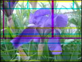
Example: An image which has been decomposed at discontinuous points along each of its three color planes (n.b.: this is why some cells seem to overlap, and why the border of the highlighted cells are of different colors):